- Posted on
- Accelity Marketing
- 0
Introduction
An FX Carry Trade is a popular currency investment strategy that involves borrowing money in a currency with a relatively low interest rate and investing that money in another currency with a higher interest rate. For example, assume the market interest rate in Japanese Yen (JPY) is 1% and the interest rate in the Australian Dollar (AUD) is 6%. A carry trade strategy would borrow JPY at 1% interest, instantly convert it into AUD, and invest the proceeds at the 6% rate. At the end of the trade period, the original investment plus the 6% return in AUD is converted back to JPY to pay off the 1% interest on the loan. If the exchange rate remains unchanged over the period, the profit of the strategy would be the 6% return minus 1% interest, or 5%. Generally, since the AUD interest rate is higher than the JPY rate, there is an expectation that the AUD will weaken and depreciate relative to the JPY. In practice, that depreciation is usually less than the profit made from the interest rate differences.
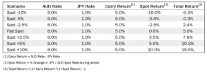
Figure 1 – Sample Carry Trade AUD vs JPY
The chart above demonstrates the profits from an AUD / JPY example trade with varying spot exchange rate changes between -10% to +10% over the period. For example, if the spot exchange rate goes down 2.5%, the trade still makes a 2.4% profit. However, if the spot exchange rate goes down 5% over the period the profit is wiped out to a 0.3% loss. There is also a possibility of an appreciation of the currency which would increase the profitability of the trade.
Individual Currency Study
Our individual currency carry trade study analyzed a group of 33 currencies over a historical period from January 1st, 2000 to December 31st, 2019 to measure the profitability of each currency pair trade. The table below shows a summary of the results for the carry trades using the USD and each of the 32 other currencies.
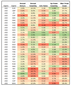
Figure 2 – Results of Individual Currency Pairs vs USD
Based on the table above, one could conclude that the best strategies would use the Argentine Peso (ARS) or Turkish Lira (TRK) since they had the highest annual return over the time period (9.6% and 6.3%). However, looking at only the expected returns ignores other important risk measures of the trade such as volatility and maximum drawdown. The five measures our study looked at are listed below.
Annual Return: The annualized percent return over the period from 2000-2019. This provides a raw measure of the profitability of the trade.
Annual Volatility: The annualized standard deviation of the returns over the period from 2000-2019. This provides a measure of the risk of the trade.
Information Ratio: The Annual Return divided by the Annual Volatility. This provides a measure of the return relative to the risk of each trade and is a good way to directly compare amount of additional return achieved for taking on additional risk.
Up to Down Volatility: The volatility on trades with positive returns divided by he volatility on trades with negative returns. This measures the dispersion of results on positive trades relative to that of negative trades. A higher value is favorable and implies a lower probability of a large loss that will wipe out profits.
Max Drawdown: The maximum loss from the highest point of an investment before a new high point is attained. It is an important measure of capital preservation. A lower historical max drawdown implies that the strategy is less likely to suffer large losses that wipe out profits.
Portfolio Study
Individual carry trades can be profitable but, as demonstrated above, take on the exchange rate risk of the currency pair. By utilizing a portfolio of currencies optimized based on expected returns, volatility, and correlation, a portfolio strategy can be used to achieve relatively good expected returns while minimizing risk through the diversification and hedging of exchange rate risk. Our study implemented an optimized portfolio strategy and backtested historical results from 2000-2018 using three different currency groups paired with the USD and a few other modeling assumptions.
A33: All 33 currencies in the study.
G10: The G10 currencies – EUR, GBP, JPY, CHF, SEK, DKK, NOK, CAD, AUD, and NZD.
E23: The 23 Non-G10 currencies – CNY, HKD, INR, IDR, PHP, SGD, KRW, TWD, THB, CZK, HUF, ISK, PLN, RUB, SKK, TRY, ZAR, ARS, BRL, CLP, COP, and MXN.
Assumptions: Target Volatility: 5.0%, Maximum Currency Weight: +/-0.5 for G10 and +/-0.3 for A33 and E23, Maximum USD Total Weight: +/- 0.5, Maximum Absolute Value of Weights: 3.0 and Rebalancing Period: Monthly. In addition to the interest and exchange rate of each currency pair, an estimate of the volatility and covariance of each currency is necessary to optimize the trading strategy to meet the target volatility. The first and simplest method is to calculate historical volatility by looking backwards a certain number of days for each trading period. A second method called GARCH, or Generalized AutoRegressive Conditional Heteroskedasticity, assumes that the variance is a random process and uses a fairly complex procedure to calculate the variance at each trading period. Our study analyzed a group of scenarios that included the historical and GARCH methods and used a calculation look back period from 30 to 360 days. The table below shows the results for different variance calculation procedures using the A33 group.
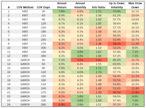
Figure 3 – Results of Variance Scenario Analysis A33 Portfolio
Based on the above analysis, the GARCH method doesn’t appear to add value based on the five parameters. It also appears that a variance look back period around 300 days starts to maximize our information ratio and minimize the max drawdown without being excessively long. For comparing the three portfolio strategies in our study, a historical volatility will be used with a calculation look back period of 300 days. Using those assumptions for the currency variance and correlation, along with monthly re-balancing of trades and a target portfolio volatility of 5%, the results of the three portfolio strategies are shown below.
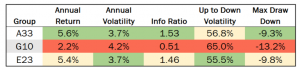
Figure 4 – Portfolio Analysis: Historical 300 Day Variance
Both the A33 and E23 optimized portfolio strategies provide annualized returns of around 5.5% with information ratios of about 1.5 while the G10 strategy looks less favorable with an annual return of only 2.2% and information ratio of only 0.51. From 2001-2019, the S&P 500 had an annualized return of 5.23% with an information ratio of 0.29 and a maximum drawdown of 56.8%. Based on our study, the A33 and E23 carry trade strategies perform favorably in comparison and warrant further analysis and consideration.
Figure 5 – Portfolio Strategies vs. Benchmark
ADDITIONAL CARRY TRADE ANALYSIS
AtlasFX has performed analysis on a number of other interesting components related to the carry trade and works directly with clients on managing their foreign exchange risk. A few additional areas of study are shown below. Please inquire with us directly about additional details on the study.
GDP WEIGHTS PORTFOLIO ANALYSIS
In our initial study, the maximum weights for each currency were 0.5 for G10 and 0.3 for the A33 and E23 strategies. To enhance the analysis and make it more realistic for clients with FX risk spread across the globe, we applied a new set of maximum weights for each currency based on GDP. Below is a table showing the maximum weights for each currency used in this new analysis.
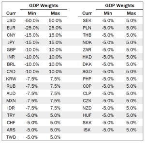
Figure 6 – Currency Weights Based on GDP
By limiting the weights in the smaller, riskier currencies the strategy sacrifices some of the large expected returns in favor of a less volatile and more realistic strategy to implement. The table below shows the results of the three portfolio strategies using the GDP weights.
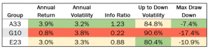
Figure 7 – Portfolio Analysis: Historical 300 Day Variance
The A33 and E23 carry trades still perform at high information ratios of 1.23 and 0.88 and small maximum drawdowns of 7.4% and 17.4%. These strategies also perform comparably on an expected return basis to the S&P 500 and MSCI World Index and warrant consideration for a firm with significant FX exposure. Atlas FX works with its clients on custom FX risk and investment strategies.
Figure 8 – GDP Weight Portfolio Strategies vs. Benchmark
INDIVIDUAL PAIRS ANALYSIS
Our study analyzed a universe of 33 currencies paired with the USD and each other. A few sample figures are shown below.
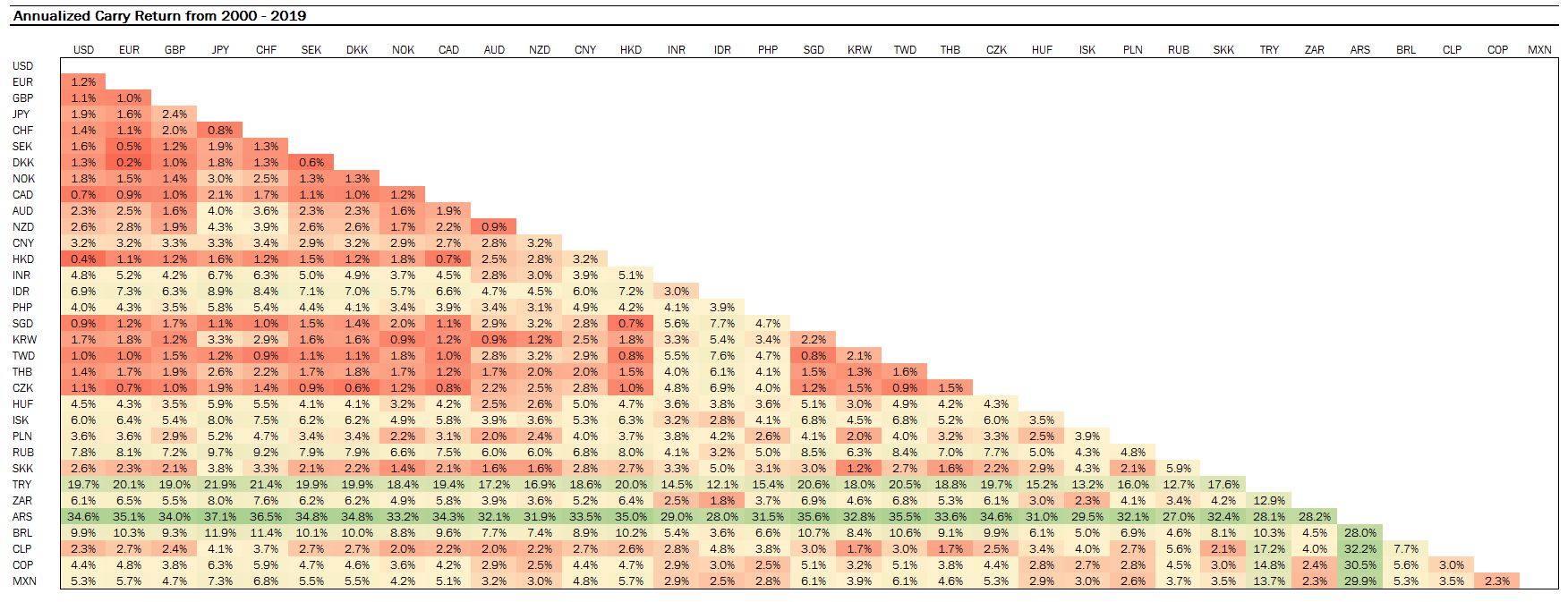
Figure 9 – Matrix of Annual Returns – All Currency Pairs (click to enlarge)
Figure 10 – Individual Currency Pair Charts
HISTORICAL SPLITS (2000-2005, 2006-2011, 2012-2019)
We split our analysis into three historical periods to view how the strategies’ performances may vary over time. For almost every currency pair the period from 2000-2005 performs better than the more recent periods.
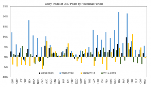
Figure 11 – Historical Returns by Time Period Chart
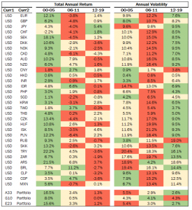
Figure 12 – Historical Returns by Time Period Table
PREDICTIVE VALUE OF CARRY RETURN TO TOTAL RETURN
Do higher carry returns result in a higher overall return? We analyzed the relationship between the carry return and the total return of all 529 currency pairs to show there is a positive relationship with a correlation of 67% and an R-squared of 0.4448. A sample chart is shown below. The relationship does hold, although it may not be as strong as anticipated.
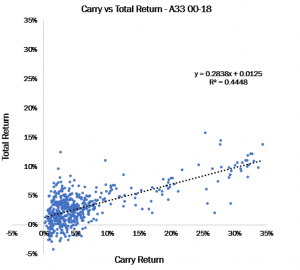
Figure 13 – Linear Regression of Carry Return vs. Total Return (including Spot)